54 sorting interview questions [easy, medium, hard]

To ace your coding interview for a software engineering job, you’ll need to understand sorting. It is fundamental to many other algorithms and forms the basis of efficiently solving many problems, from CPU optimization to searching and data retrieval. 

Here are some typical questions that involve sorting:

Below, we take a look at 54 sorting questions and provide you with links to high quality solutions to them. 

This is an overview of what we’ll cover:

1. Easy sorting interview questions
2. Medium sorting interview questions
3. Hard sorting interview questions
4. Sorting basics
5. Sorting cheat sheet
6. How to prepare for a coding interview

Let's get started.

Click here to practice coding interviews with ex-FAANG interviewers

1. Easy sorting interview questions

You might be tempted to try to read all of the possible questions and memorize the solutions, but this is not feasible. Interviewers will always try to find new questions, or ones that are not available online. Instead, you should use these questions to practice the fundamental concepts of sorting.

As you consider each question, try to replicate the conditions you’ll encounter in your interview. Begin by writing your own solution without external resources in a fixed amount of time.

If you get stuck, go ahead and look at the solution, but then try the next one alone again. Don’t get stuck in a loop of reading as many solutions as possible! We’ve analysed dozens of questions and selected ones that are commonly asked and have clear and high quality answers.

Here are some of the easiest questions you might get asked in a coding interview. These questions are often asked during the “phone screen” stage, so you should be comfortable answering them without being able to write code or use a whiteboard.

2. Medium sorting interview questions

Here are some moderate-level questions that are often asked in a video call or onsite interview. You should be prepared to write code or sketch out the solutions on a whiteboard if asked.

3. Hard sorting interview questions

Similar to the medium section, these more difficult questions may be asked in an onsite or video call interview. You will likely be given more time if you are expected to create a full solution.

4. Sorting basics

In order to crack questions about sorting, you’ll need to have a strong understanding of the concept, how it works, and when to use it.

4.1 What is sorting?

Many algorithms require, or perform better on, a sorted dataset. Take searching as an example: to search an unsorted dataset of 1,000 items means looking at all 1,000 items in the worst case. In contrast, using binary search on a sorted dataset of 1,000 items means looking at 10 items in the worst case. For a bigger dataset of 1,000,000 items, searching it as unsorted is looking at 1,000,000 items at worst, but searching it as sorted is looking at 20 items at worst. Being able to sort data effectively can therefore yield returns later in an algorithm.

Sorting can be performed on arrays or linked lists. Our examples will be based on the following array:

8, 5, 7, 4, 2, 1, 3, 6, 9, 3, 1, 5, 2, 4, 6

Insertion sort

Insertion sort is one of the simpler sorting algorithms. It works with both arrays and linked lists. The data structure can be imagined as being split into two parts: a sorted part, followed by unsorted items. The first item in the unsorted part is moved to its correct position in the sorted part. In the image below, the first two iterations of insertion sort are shown.

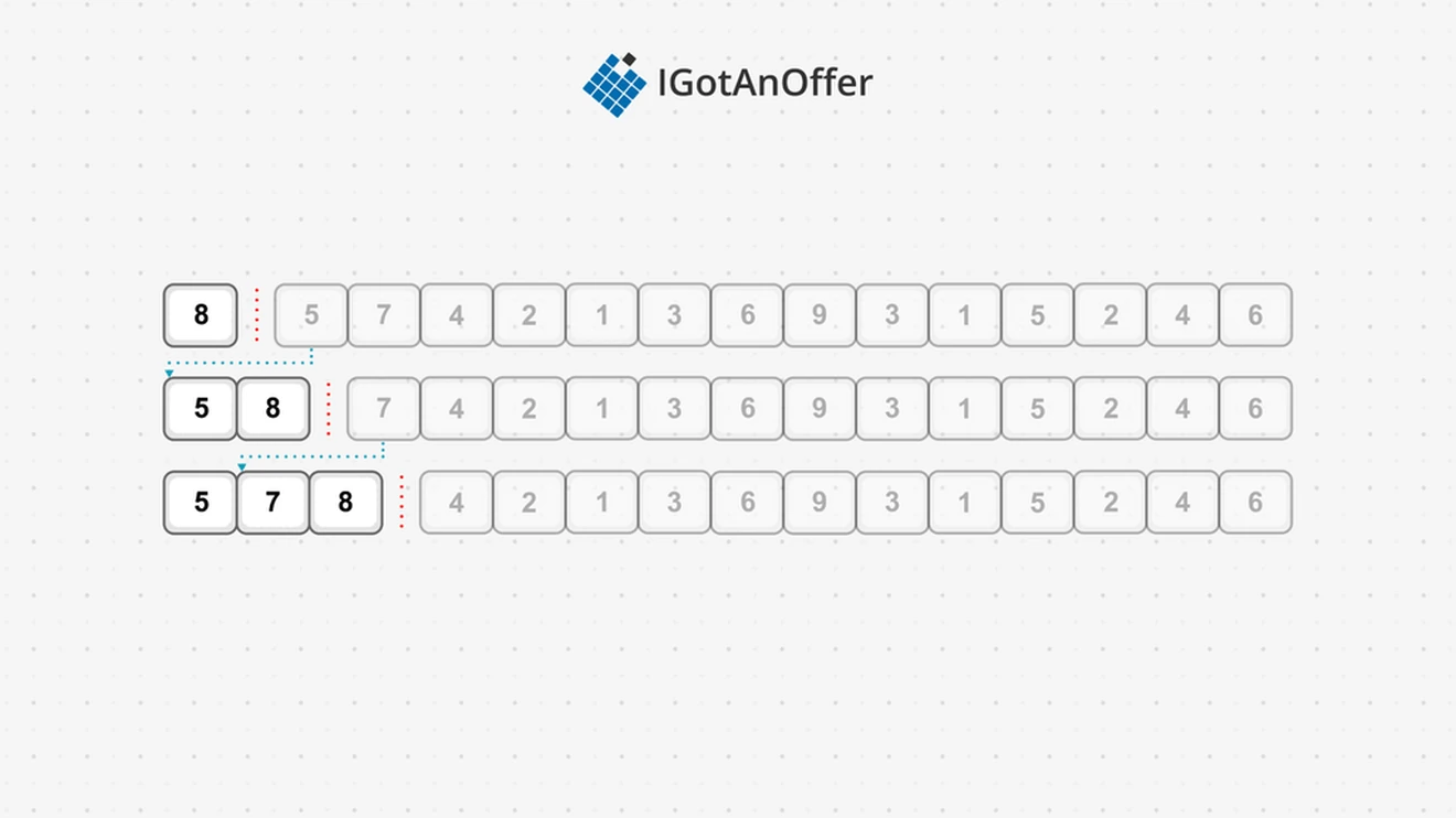
There is an invisible divide between the first element with the value 8, and the second element with the value 5. Everything before the divide is sorted and everything after the divide is unsorted. On the first iteration, the first item from the unsorted set, the 5, is placed in the correct position in the sorted set. Since 5 is less than 8, the 5 will be placed before the 8 at index 0. All the elements from this index 0 to the end of the sorted subset need to be moved along by one position. In this instance, 8 moves one position to the right, and the 5 is placed at index 0. On the next iteration, the 7 is to be inserted into its correct position at index 1. Everything after index 1 in the sorted set moves one position to the right, and the 7 is placed at index 1.

Now imagine a list of 1,000 items, and the last iteration needs to insert an item at index 2. All 997 items that follow index 2 will need to move one position up, which could potentially take O(n) time for each iteration. This demonstrates how insertion sort is impractical for big data structures.

Quicksort

Quicksort also works on both arrays and linked lists, and uses a pivot item to divide the data structure in two: those items with a value less than the pivot item, which are placed in front of the pivot, and those with a value greater than the pivot, which are placed after the pivot. Each of the two sets is then sorted with Quicksort.

The pivot is usually the item in the middle of the list for the array implementation, but the last item for the linked list implementation.

Here we show the first 3 three iterations of Quicksort on our earlier array:

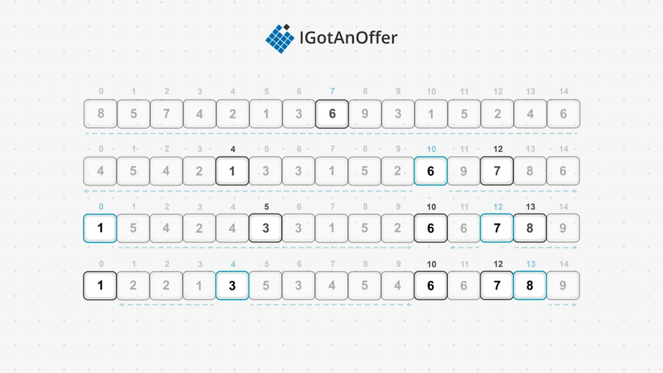
The pivot item is in the middle of the array at index 7, with a value of 6. After the first iteration, all items smaller than 6 will be placed to the left of it, and all items larger to the right. Our 6 is now in its correct position in the sorted array, at index 10.

Notice that the algorithm has created two subarrays: one spanning indices 0-9 and the other indices 11-14. Quicksort is now performed on the subarrays: the pivot of indices 0-9 is at index 4 with the value 1, and the pivot of indices 11-14 is at index 12 with the value 7. When both subarrays have been sorted, the 1 and 7 are also in their correct positions. In this iteration, only one subarray is created for each of the two subarrays created in the first iteration. There are no subarrays to the left of 1, and the subarray to the left of 7 has a length of 1, so it will not be sorted. With the third iteration, the 3 and 8 are placed in their correct positions.

Each iteration has some work to do to move the items to before or after the pivot. Here’s what it does:

1. Determines the pivot index and swaps its value with the first item.
2. Initializes a smallIndex variable to 0. This variable will mark the boundary between items smaller than the pivot item and those greater than the pivot item.
3. Loop through the array starting at the second item. If the current item is smaller than the value of the pivot, then increment smallIndex and swap the item at the new smallIndex with the current item.
4. Swap the pivot, at index 0, with the item at smallIndex.

Here is an example of the first iteration of Quicksort after the pivot item 6 has been swapped with the first item 8.

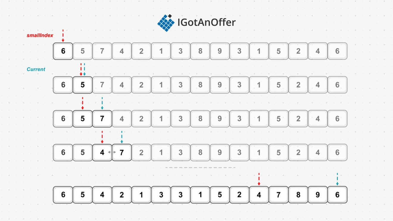
First, smallIndex is initialized to 0. The loop starts from the second item, which is at index 1 and has a value of 5. Since 5 is smaller than the pivot item, which has a value of 6, smallIndex increments to index 1, and the item at index 1 (smallIndex) is swapped with the item at index current. Since smallIndex and index current are both index 1, the 5 swaps with itself. On the next loop, the 7 is determined to be greater than the pivot (which has a value of 6), so only current increments to index 3. On the next loop, 4 is smaller than the pivot, so smallIndex increments to index 2 and swaps with the current value - the 4 and the 7 swap. This continues until the last iteration, when smallIndex will have the value 10 and the loop exits. Now the 4 at index 10 swaps with the pivot to end the iteration and give the result shown in the first graph of this section.

Quicksort is known as a divide-and-conquer sort, since the list is divided into smaller lists that are easier to manage. Each small list in turn is made smaller, and with each iteration, the pivot is placed at its correct position.

Mergesort

Mergesort is another divide-and-conquer sort algorithm for arrays and linked lists. It works by breaking down an unsorted list into single elements, and then recombines them in order.  The algorithm for mergesort works as follows:

1. Divide the list into two sublists
2. Mergesort the first sublist
3. Mergesort the second sublist
4. Merge the two sublists into one bigger sorted list

Most of the work of mergesort is done in step 4 when the lists are merged.

Here’s a visual of steps 1 to 3 performed on our example array:

First, the array is divided into two: an array of size 7 and one of size 8. Next, these two subarrays are divided into two arrays each, with sizes of 3, 4, 4, and 4. Subarrays continue to be divided in two, until all subarrays have a size of 1. Then step 4 merges the subarrays.

The process of merging two arrays together is as follows:

1. Initialize two pointers, pointer a to zero (0) for indexing the first sublist and pointer b to zero (0) for indexing the second sublist.
2. While a or b has not reached the end of their respective lists, move the items as follows:
   - If the item at list1[a] is smaller than the item at list2[b], then push list1[a] to the merged array and increment a.
   - Else push list2[b] to the merged array and increment b.
3. Once at least one of the two pointers has reached the end of its list, append the remaining items in the other list to the merged array.

Below is an example of merging two subarrays that are already sorted:

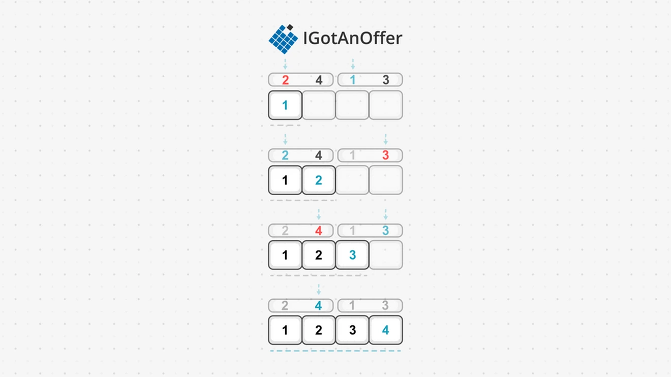
The loop starts for both sublists, and the pointer b at the second sublist has the smallest item with a value of 1. This value, 1, is added to the merged list at index 0, and b is incremented to index 1. Next, the value 2 at pointer a is smaller than the value 3 at pointer b, so it’s placed in the merged list at index 1, and a is incremented. The value of 3 from sublist 2 is the next smallest item that is moved to the merged list. Sublist 2 is now exhausted and the loop ends, but since sublist 1 still has items in it, they are all moved to the merged list.

Heapsort

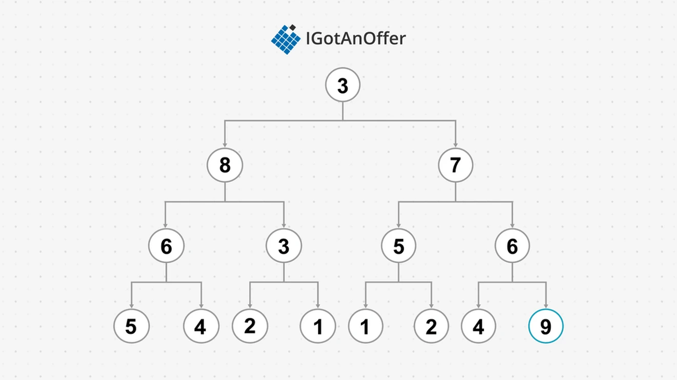
Heapsort takes an entirely different approach to sorting arrays and linked lists. Heapsort uses the concept of a priority queue, which will pop the biggest item in the queue at speed. This item is then pushed to the end of the array, and the next biggest item is popped and added to the second-to-last position in the array. This continues recursively until the priority queue is empty. Like insertion sort, heapsort divides its list into a sorted section and an unsorted section. The sorted section is at the end of the list and the unsorted section is in a special structure called a heap. A heap is visualised as a binary tree, but generally stored in an array.

A heap is when any item at index i is bigger than the items at index 2i + 1 and 2i + 2. Our example array is not in a heap because the value 4 at index 3 is not greater than the value 6 at index 7 (2*3 + 1), nor the value 9 at index 8 (2*3 + 2).

To build and maintain a heap, two operations are used: heapify-up and heapify-down.

For a better understanding of heaps, take a look at the heaps article in our data structure series.

The result of performing a heapify operation on the unsorted section of our example list is that the unsorted section will satisfy the heap property. Even though heapsort will operate on an array, it’s easiest to imagine the heap as a tree in which every parent node has a value greater than that of its children, and the root (index 0) will contain the item with the greatest value.

Heapsort then sorts the data by swapping the item at the root (index 0) of the heap with the last item of the array. This places the root item in its correct location in the sorted section, and the unsorted section is reduced by one item.

Since the unsorted section no longer satisfies the heap property, a heapify-down operation is performed, and the item with the greatest value in the unsorted section will be at the root of the heap, or index 0. This item is then swapped with the second-last item of the array, placing it in its correct location in the sorted section, and reducing the unsorted section by one item again. Heapify is performed again so that the unsorted section satisfies the heap property, and the process can be repeated until the unsorted section is exhausted.

Here is the first iteration of heapsort after the root node of our heap is swapped with the last item in our array:

Now the value 9 is in its correct position at index 14, and only indices 0-13 form the heap. Since the heap property is broken, the 3 at index 0 will swap with the 8, then with the 6, and finally with the 5 in a heapify-down operation, placing 8 at index 0. The 8 at index 0 is swapped with the 4 at index 13, placing it in its correct location in the sorted array, and indices 0-12 are heapified. This continues until all the items in the array are sorted.

Counting sort

All the algorithms discussed so far are called comparison sorts, since they compare the items in a list with each other. No comparison sort algorithm can ever perform better than O(n log_2 n), so other algorithms exist to overcome this. Counting sort is one of them.

Counting sort uses an intermediate array to calculate the final index for each item in the sorted array. This array is built as follows:

1. Find the max number in the unsorted array.
2. Create the temporary array temp, with length=max and initialize all indices to zero (0).
3. Loop over the unsorted array. For the current item, increment the index corresponding with its value in the temp array by 1.
4. Loop over the temp array to transform it into a cumulative count. Make index i cumulative using temp[i] += temp[i - 1].

Applying these steps to our example array results in the following temp array that has 9 indices, since 9 is the biggest number in the array:

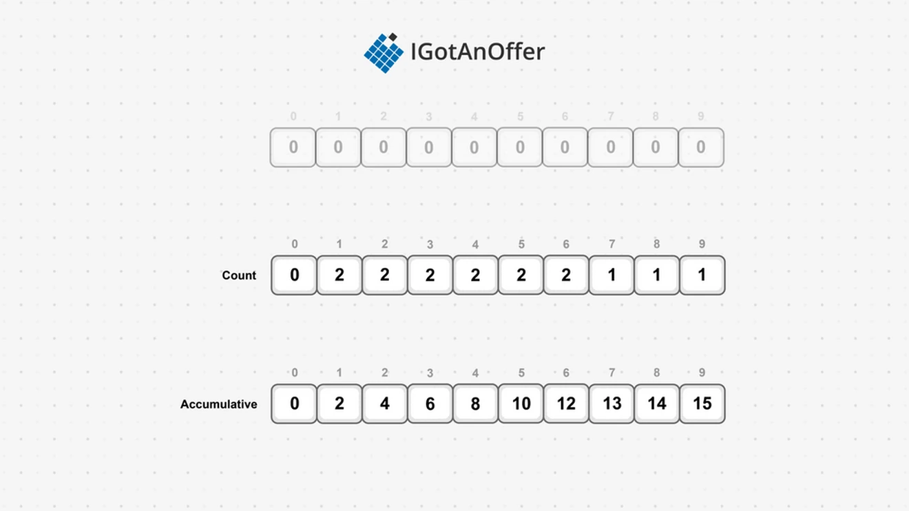
Since 1 appears twice in our example array, the index 1 in temp gets a count value of 2. The value 8, however, only appears once, so index 8 has a count value of 1.

When counting is complete, the counts are accumulated. Index 1 and index 2 have a count of 2 each, so the accumulated value of index 2 is 4. Index 3 has a count of 2, which is added to the accumulated value for index 2, which is 4, giving index 3 an accumulated value of 6.

This array can now be used to move each item in the unsorted array into its correct position in a new sorted array. This is done by looping over the unsorted array in reverse, and doing the following:

1. For the current value, find its accumulated count in the temp array at the index of the value.
2. Decrement this count value by 1.
3. Use the new count value as an index in the sorted array to store the current value

For our example unsorted array and its accumulated array, this will produce a sorted array as follows:

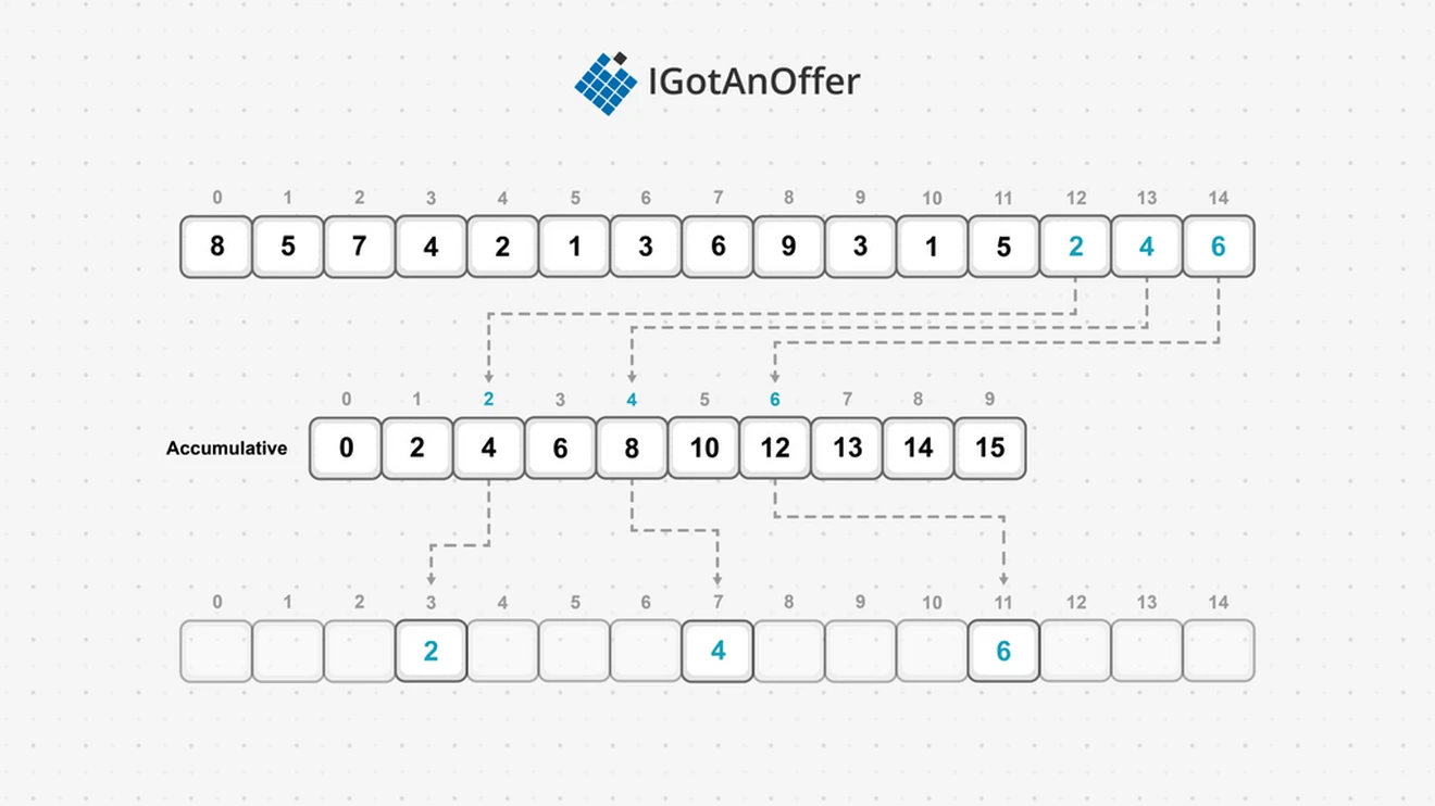
Starting at the end, index 14 (with the value of 6) has an accumulated count of 12 in the accumulated array. By decrementing one from 12, index 11 is identified as the correct position for the value 6 in the sorted array. Next, the 4 has an accumulated count of 8, so after decrementing to 7, index 7 houses the 4. On the third iteration, the 2 has an accumulated count of 4, which gets decremented to 3, so index 3 will house the 2.

4.1.1 Use cases for sorting

Sorting makes other algorithms possible or easier:

• Binary search needs its array to be sorted.
• Removing duplicates from a list is easier when the list is sorted, since the duplicate items will be consecutive items in the sorted array.
• Comparing two lists for equality is easier if they are both sorted, since the item at each index will then be equal.
• Some priority queue algorithms need a sorted list.
• It is used to solve the inversion count problem.

4.1.2 Example implementation

Some of the following example implementations use the following helper function to swap two elements in an array:

Insertion sort

The for loop is used to track the invisible divide between the sorted and unsorted parts using first_out_of_order. If the first item in the unordered set is bigger than the last item in the ordered set, then nothing more is needed for this iteration. Else, the first item in the unordered set is stored in tmp and a while loop is used to move all the items in the ordered set one position right until the position, variable i, for tmp is found.

Something to note: the for loop starts at index 1 and not index 0, as an array with only one element can be regarded as sorted.

Quicksort

The heavy work for Quicksort is done in partition, which finds the pivot in the array and moves all the elements smaller than the pivot to its left and everything greater than the pivot to its right. Finally, the pivot position is returned for the next recursive call in rec_quicksort, which will recurse into the subarrays to the left and the right of the pivot. The recursive function is wrapped with quicksort to make client calls easier.

Something to note is the special calculation of middle to prevent integer overflows.

Mergesort

In mergesort, the bulk of the algorithm’s work is done in merging the arrays. First, the smallest items from the two arrays are compared and placed until one of the two arrays runs out of items. Then all the remaining items of the non-exhausted array are placed. The function mergesort will call this merging process each time it needs to join two sorted arrays together.

Heapsort

The function heapify is an implementation for the heapify-down step. In the while loop, the parent, stored in tmp, is pushed down whenever it is smaller than its largest child. Rather than swapping parent and child with each iteration, the parent is stored in tmp, and the children are moved up as many times as necessary, and tmp (the parent) takes the place of the last opened child. This is an optimization to reduce the number of swaps.

The first loop in heapsort is the heapify-up operation and the second loop does the sorting work of moving index 0 (the biggest element) to the end of the heap and then restoring the heap property with a heapify-down operation.

Counting sort

This function initializes the accumulative array to the correct size. The first loop does the counting for each value and the second loop does the accumulation. The accumulation array is then used to move each item to its correct position in a temporary array. Finally the temporary array is copied over the original array.

4.1.3 How sorting compares to other algorithms

The sorting algorithms described here are a small sample of the wide variety of sorting algorithms that exist.

There are simpler sorting algorithms, like bubble sort, but bubble sort’s poor performance means it is only used when a simple implementation is needed. The same applies for selection sort. For this reason, Quicksort and Mergesort are more likely to be used in practice. Sample sort, a modification of Quicksort, can be used to improve how well Quicksort can be run in parallel. The idea is to take a sample of items from the list and put them in a bucket. Each bucket is then sorted on its own thread.

Sorting a range from 1 to 1,000,000 using counting sort creates a temporary cumulative array of 1,000,000 items. This is a big space requirement, and the more specialized radix sort can be used to reduce the space required. In radix sort, some base number is chosen, for example 10, and sorting happens from the least significant digit to the most significant. In other words, sorting will only look at the one digit for each item, then at the ten digit of each item, then at the hundred digit of each item, and so on. When using base 10, these digits only run from 0 to 9, so the temporary cumulative array will only have a length of 10. Radix sort therefore recursively uses counting sort, making it another non-comparative sort.

Insertion sort works best for short arrays, since all the values may need to be moved, so Timsort is an alternative when working on longer arrays. Timsort divides an array into smaller arrays, called runs, with lengths of between 32 and 64 elements. These subarrays are sorted with insertion sort, and mergesort is used to form a sorted big array from these small sorted arrays.

5. Sorting cheat sheet

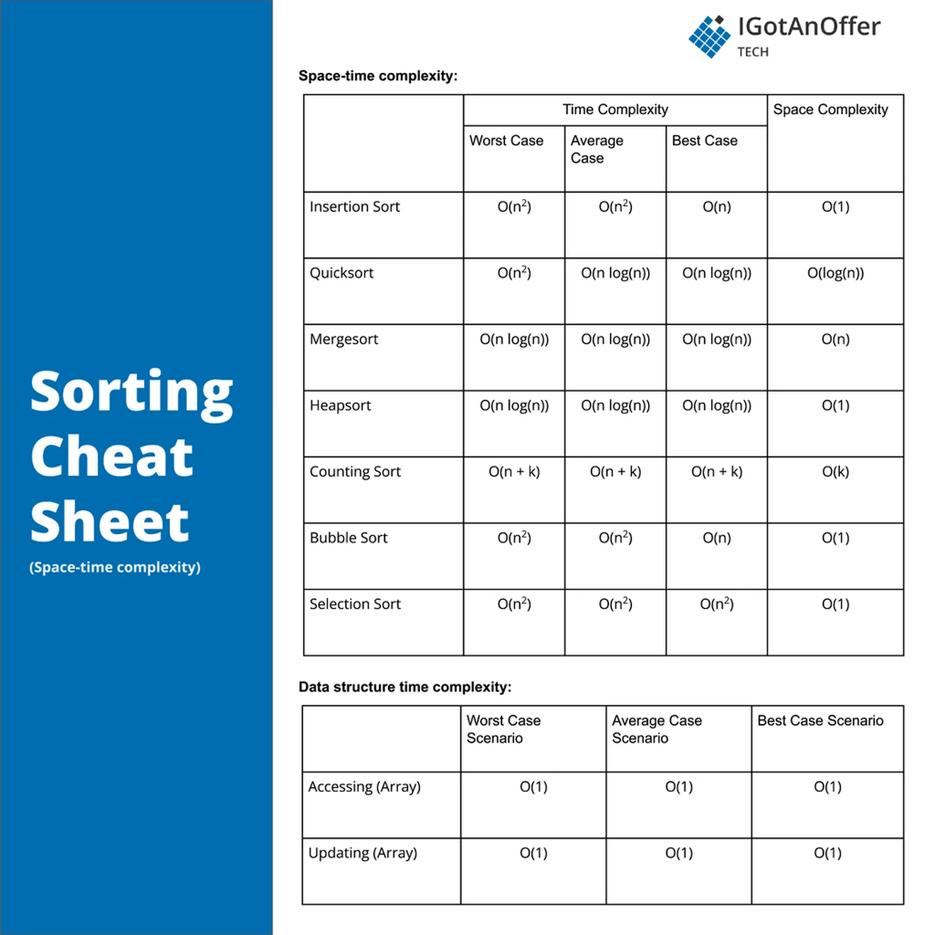
You can download the cheat sheet here.

5.1 Related algorithms and techniques

• Two pointers

• Priority queue

• Timsort

• Radix sort

• Pigeonhole sort

• Smoothsort

5.2 Cheat sheet explained

The cheat sheet above is a summary of information you might need to know for an interview, but it’s usually not enough to simply memorize it. Instead, aim to understand each result so that you can give the answer in context.

The cheat sheet is broken into time complexity and space complexity (the processing time and memory requirements for sorting). Sorting is related to several data structures, which are also included in the cheat sheet.

For more information about time and space requirements of different algorithms, read our complete guide to big-O notation and complexity analysis.

5.2.1 Time complexity

Insertion sort has two nested loops to give a time complexity of O(n^2), and only the inner while loop can stop early when the list is already sorted, giving a best case of O(n).

In the worst case, Quicksort might select a pivot that is the smallest or largest item with each recursion. This will cause each recursion to operate on i - 1 items for n recursion times. In the end this gives a O(n^2) worst time complexity. The best case divides the list perfectly (meaning no elements need to be moved) for a recursive depth of log_2(n) and each level will process n items for a best case complexity of O(n log_2 n). The average complexity is also O(n log_2 n).

Mergesort does a perfect division on each recursive call to give a total of log_2(n) recursive calls. When merging two sublists together, a total of n items needs to be moved to the merged list for each recursive call, giving a time complexity of O(n log_2 n). These exact steps happen for the worst, average, and best case.

Heapsort uses the heapify function to build the heap and keep it sorted, and heapify loops through the list, as if the list is a tree, from parent to child to give log_2(n) loops. Building the heap runs a loop for n/2 times, calling heapify each time. And the sorting runs n times, also calling heapify each time. This gives a total time complexity of O(n log_2 n) for the worst, average, and best case.

Counting sort loops over the array three times: once to build the accumulated array; once to move each item to its correct position in the temporary array; and once to move the items from the temporary array to the sorted array. This is a total of 3n operations, but the accumulated array has k items, where k is the maximum value in the original array. There is one loop over the accumulated array to turn the counts into an accumulation, and this loop has k - 1 iterations. This gives a total time complexity of O(n + k) in the worst, average, and best case.

5.2.2 Space complexity

Insertion sort reuses the original array for a space complexity of O(1). However, insertion sort has a bad swapping performance since swaps happen inside a nested loop. This gives an average and worst swap case of O(n^2), and a best case of O(1) when the list is already sorted.

Quicksort also reuses the original array for O(1) space complexity, but it also includes many swaps. In the worst case, for a reverse-sorted list, the pivot could be the biggest item with each iteration, causing n - 1 recursions. Since the pivot is the biggest item in the list, there will be i swaps for a total of O(n^2) swaps. The best case chooses a perfect pivot for log_2(n) recursions and thus also n swaps on each recursion for a swap of O(n log_2 n). The average case is also O(n log_2 n) swaps.

Mergesort has a temporary array for each merge operation, and the merge operations happen layer by layer with n items in each layer. This gives mergesort a space complexity of O(n). In terms of swaps, mergesort has log_2(n) recursions with n swaps on each recursion. So there are O(n log_2 n) swaps in the worst, average, and best case.

Heapsort reuses the original array for a space complexity of O(1). In terms of swaps, heapsort will call heapify n/2 times to build the heap, and then n times to sort the list in the worst, average, and best case. In the best case, the list might be entirely sorted, so no swaps are needed when building the heap, but log_2(n) swaps will be needed during the sort. The worst case has the list unsorted and will need log_2(n) swaps in the build process and another log_2(n) swaps in the sort process. In total, the number of swaps needed are O(n log_2 n) in the worst, average, and best case.

Counting sort uses a temporary array with n items and an accumulated array with k items, where k is the maximum value in the array to be sorted. This gives a total space complexity of O(n + k). In terms of swaps, each item gets moved directly to its correct position in the temporary array and then back to the original array for a total number of O(n) swaps in the worst, average, and best case.

5.2.3 Sort implementations (Java, Python, C++)

The “sort” function from the C++ STL does not subscribe to a specific sorting algorithm, only requiring that the algorithm performs better than O(n log n). The worst case of Quicksort does not meet this requirement; however, C has a function called “qsort” that does implement Quicksort and “qsort” is in the standard C library of C++.

Timsort was specifically created by Tim Peters to be the sorting algorithm for Python in 2002. Calling “sort” since Python 2.3 uses Timsort. Java also used a variant of Timsort when sorting objects since Java 7.

6. How to prepare for a coding interview

6.1 Practice on your own

Before you start practicing interviews, you’ll want to make sure you have a strong understanding of not only sorting but also the rest of the relevant algorithms and data structures. You’ll also want to start working through lots of coding problems.

Check out the guides below for lists of questions organized by difficulty level, links to high-quality answers, and cheat sheets.

Algorithm guides

• Breadth-first search
• Depth-first search
• Binary search
• Dynamic programming
• Greedy algorithm
• Backtracking
• Divide and conquer

Data structure guides

• Arrays
• Strings
• Linked lists
• Stacks and Queues
• Trees
• Graphs
• Maps
• Heap
• Coding interview examples (with solutions)

To get used to an interview situation, where you’ll have to code on a whiteboard, we recommend solving the problems in the guides above on a piece of paper or google doc.

6.2 Practice with others

However, sooner or later you’re probably going to want some expert interventions and feedback to really improve your coding interview skills.

That’s why we recommend practicing with ex-interviewers from top tech companies. If you know a software engineer who has experience running interviews at a big tech company, then that's fantastic. But for most of us, it's tough to find the right connections to make this happen. And it might also be difficult to practice multiple hours with that person unless you know them really well.

Here's the good news. We've already made the connections for you. We’ve created a coaching service where you can practice 1-on-1 with ex-interviewers from leading tech companies. Learn more and start scheduling sessions today.