
Big-O is an important technique for analyzing algorithms. It allows software engineers to assess the time and space requirements of algorithms, and how these change in relation to the input. This means engineers can compare different algorithms and assess their suitability for specific tasks.
Below we’ll explain exactly what big-O is, how it works, and work through some examples of how to use it. We’ve also included a handy cheat sheet to help you apply big-O in some common cases.
Here’s an outline of what we’ll cover:
- Big-O and complexity analysis
- Big-O cheat sheet
- Big-O practice problems
- Why Big-O is important for FAANG interviews
- How to prepare for a coding interview
Click here to practice coding interviews with ex-FAANG interviewers
1. Big-O and complexity analysis
1.1 What is big-O?
Big-O is a method of analysis used to measure an algorithm’s performance in terms of certain properties. When we design algorithms, we need to pick the algorithm that best meets our time and space constraints. Big-O provides us with a simple expression we can use to analyze and compare algorithms.
For the most part, big-O is applied to operations performed on data structures. For an algorithm that moves items, big-O can measure the number of item copies, the amount of memory used, or the total number of coding instructions for a time-taken measurement.
When a list data structure has n elements, then the big-O for an algorithm on these elements will be in terms of n. This allows us to predict the performance of the algorithm as the input size increases by say, ten items, a thousand items, a million items, or a billion items.
1.1.1 Simplifications
Big-O does not put an exact number to copies made, memory used, or coding instructions executed in an algorithm. Instead, it focuses on the most significant elements in the measurement.
Suppose we determine n^2 to be the number of coding instructions for one algorithm (g) and n^2 +10n + 5 for another algorithm (h). The following table shows the number of instructions executed as the size of the list (n) increases.
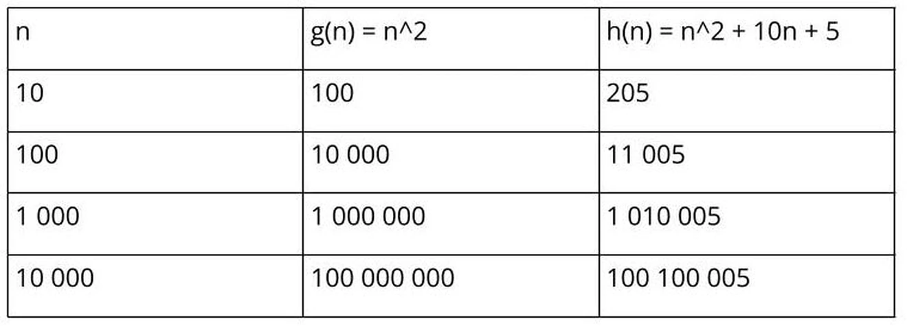
As the list reaches a thousand and more items, it is clear that the component 10n + 5 has become insignificant and can be ignored. This means the big-O analysis for both g and h is expressed as O(n^2).
The following table shows the same for an algorithm (j) having 2n memory usage and an algorithm (k) having 5n.
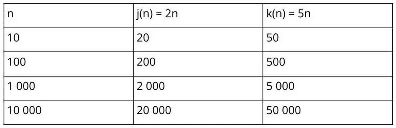
Again, the constants 2 and 5 do not make a difference in the final measurement, since n impacts the measurement the most. This means the big-O for both j and k is O(n).
In summary, for any measurement in the following form:
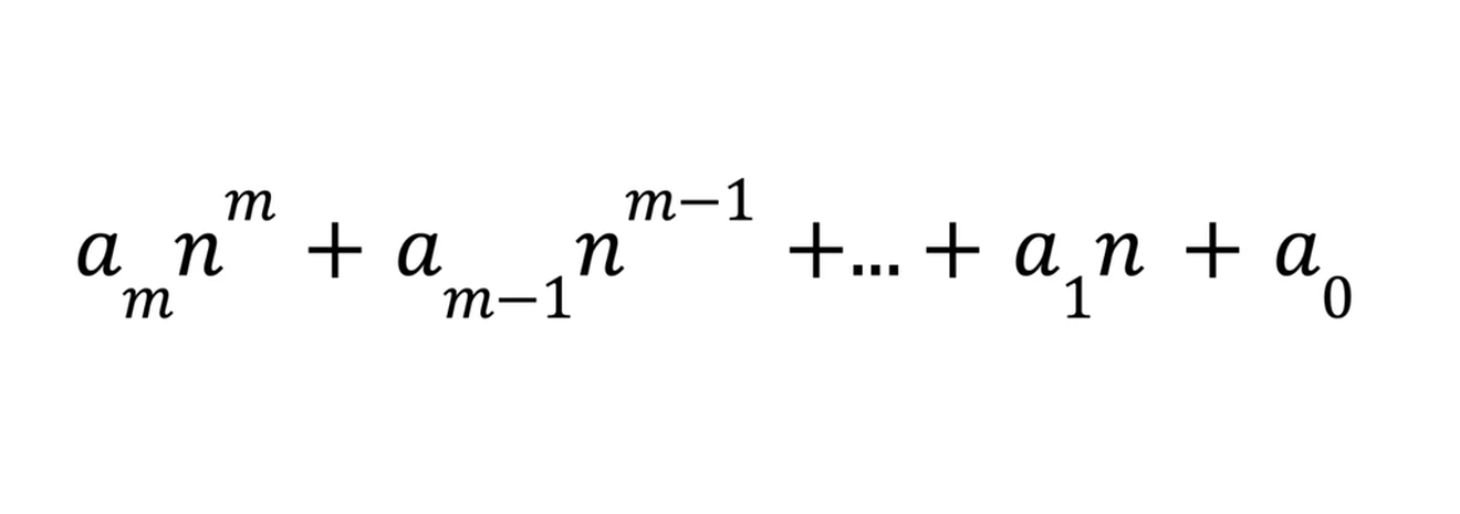
the big-O expression will be O(n^m) – the biggest term without its constant.
1.1.2 Example code analysis
Let’s examine some code to determine the big-O values, starting with the following function to get the length of a list:
This function takes in an array and does one thing: returns the size of the array. Whether the array has five or a million elements, the function performs the same single task, so the time complexity can be expressed as O(1).
The function only stores one element in memory – the length of the array – so its storage complexity is O(1). Similarly, only this one element, the length of the array, will be copied when the function returns, to give O(1) copies.
The following function returns the length of the longest word in an array:
If the array contains five words, the block of code in the for loop will run five times. Likewise, if the array contains a million words, the same block of code will run a million times. In general, for any array with n words, the loop code will run n times.
Setting the longest variable will always run once, and returning it will also always run once. This gives the function a total of n+2 instructions and a time complexity of O(n).
Our function needs memory to store the variables longest and word, and the value returned from len(). This is a total of three storage items, so this function’s space complexity is O(1). This means that the number of items stored by the function remains constant, whether the array has five or a million words.
Finding the number of copies the function needs is a bit more difficult, since copies occur on the longest = len(word) line. The number of times this line runs is dependent on the length of the words and their order in the input array to the function. But when we analyze complexity, we are mostly concerned with possible worst-case scenarios.
The worst-case here is an array in which every element at index i is longer than the element at index i-1 (every word in the array is longer than the one before it). In such a case, the line will execute for every word in the array, or n times. Since all copies outside of the longest = len(word) line are insignificant, our function has a final copy complexity of O(n).
Binary search is a common algorithm used to find elements in a sorted array by continually discarding half of the search space. Here is an example implementation of an iterative binary search:
In considering the time complexity of this example, the while loop is the significant factor. The while loop runs as long as the search space contains items, and every run of the loop halves the search space. Let’s do a worst-case analysis of this algorithm using an array of 8 elements.
The first run of the while loop will reduce the search space to 4 elements, the second run reduces the search space to 2 elements, the third run to 1 element. In the worst case, the while loop will stop and run only 3 times. In general, the while loop will run log_2(n)-1 times. Only focusing on the most significant parts gives a time complexity of O(log_2(n)).
Now for an example that does not use a data structure: finding the number of binary digits needed to store some number i. For example, the binary for the number 5 is 101, so 3 binary digits are needed to store the number 5. Here is a function to calculate this:
Here, the while loop is again the most significant factor contributing to the function’s time complexity. The variable binary doubles with each loop. This gives the same time expense as the previous binary search example. The loop will run log_2(i)-1 times, giving the function a time complexity of O(log_2(i)). The only variables stored are digits and binary, giving our function a space complexity of O(1).
Now suppose we want to find the number of binary digits for an array of numbers using the following function:
When analyzing the time complexity of this example, the loop is again the most significant factor. The loop will be called for each number in the array, a total of n times. As we saw in the previous example, the function inside the loop has log_2(i)-1 instructions. The loop means these instructions will be executed n times, so we get a total of n*(log_2(i)-1) instructions. This results in a time complexity of O(n log_2(i)), where i is the biggest number in the array.
For time and copy complexities, loops mean the multiplication of two complexities. In our example here, log_2(i) is multiplied by n. But this rule does not hold for space complexity.
For the first iteration of the loop, the inner function will use O(1) space and then the inner function will exit. On the next iteration of the loop, the same happens: O(1) space is used and then freed. The space complexity of this function is determined by how the loop affects result. By the end of the loop, result will have n numbers for a space complexity of O(n).
Let’s jump to something a bit more complex with the following code to build a multiplication table of size n:
In terms of time complexity, the loop to print the header will execute n times. This is followed by a loop to print the table, which has an inner loop. Remembering that a loop means multiplying complexities, the outer loop has n*? instructions, where ? is the number of executions within the loop. This is another loop of n executions, so the outer loop has n*n, or n^2, executions.
Instructions on the same indent level are added together for time and copy complexities. So this function has a total of n+n^2 executions – the header plus table instructions – and a time complexity of O(n^2). The space complexity is just the i and j for O(1).
As a final example, suppose you have the following brute-force password cracker – the password can only be lower case letters (26 in total) and has a length n:
The important function here is build_password to build all the possible n-length passwords. This is a recursive generator with a zero-length password as its base condition. There is an outer for loop and an inner for loop, with the outer for loop executing 26 times.
Let’s examine the inner for loop when the password has a length of 1. The base condition will be hit to give the inner loop a complexity of O(1). Combined with the outer loop, this means that for passwords of length one, the function executes 26*O(1) instructions. For a password of length two, the outer loop will execute 26 times and the inner loop as many times as needed to build a password of length 1. This is a total of 26*26 times.
And for a password of length 3, the outer loop again executes 26 times and the inner loop as many times as needed to build a password of length 2, giving 26*26*26 times or 26^3. Continuing in this way, for a password of length n there will be 26^n executions, giving the password build function a time complexity of O(26^n).
1.1.3 How big-O classes compare to one another
Big-O can be classified as follows, from fastest to slowest:
- Constant time: O(1)
- Logarithmic time: O(log n) – This includes other bases, like log_2(n), since these are essentially the changing constant. Sometimes the distinction is important and log_2(n), or its shorter version lg(n), might be written.
- Linear time: O(n)
- Linearithmic time: O(n log n)
- Quadratic time: O(n^2)
- Exponential time: O(2^n)
- Factorial time: O(n!)
The following graph shows the growth rate of these classes for a small n:
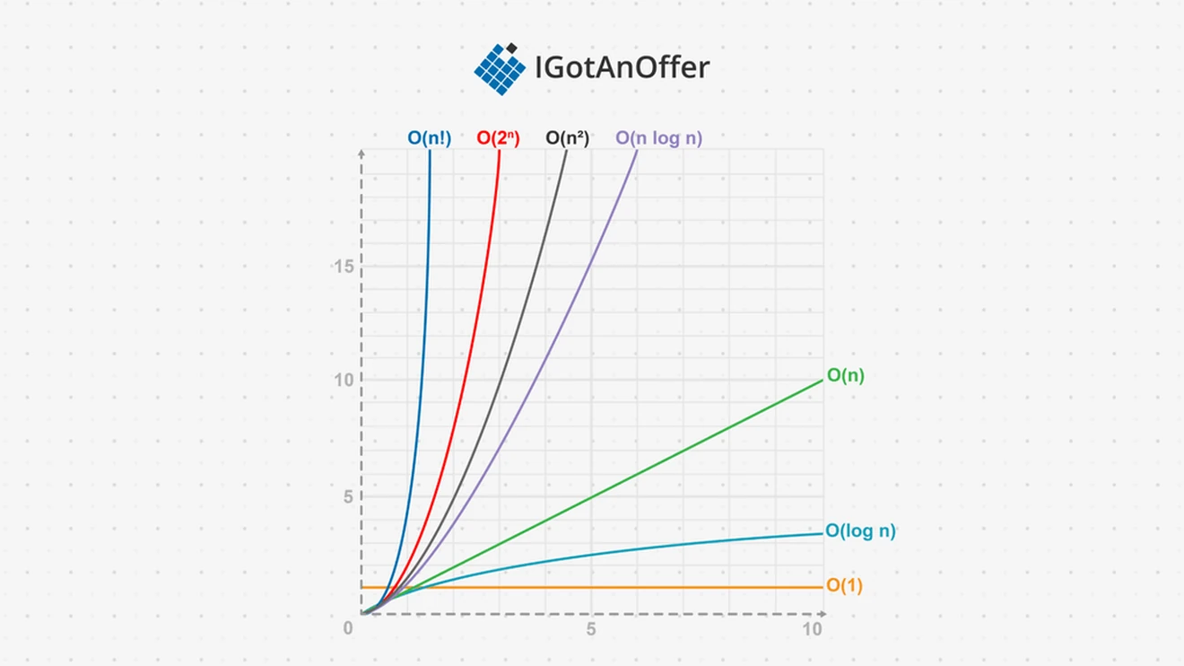
Constant time is ideal, but log and linear time is the norm. For most algorithms, linear log is acceptable, but quadratic not. Exponential time should be avoided when possible.
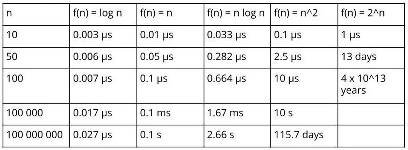
It is easier to see why we want to avoid the last two when looking at a bigger n. Suppose we have a device that can execute a billion instructions per second. The following table shows how long it will take to execute n instructions for each of these classes:
Need a boost in your career as a software engineer?
If you want to improve your skills as an engineer or leader, tackle an issue at work, get promoted, or understand the next steps to take in your career, book a session with one of our software engineering coaches.
2. Big-O cheat sheet
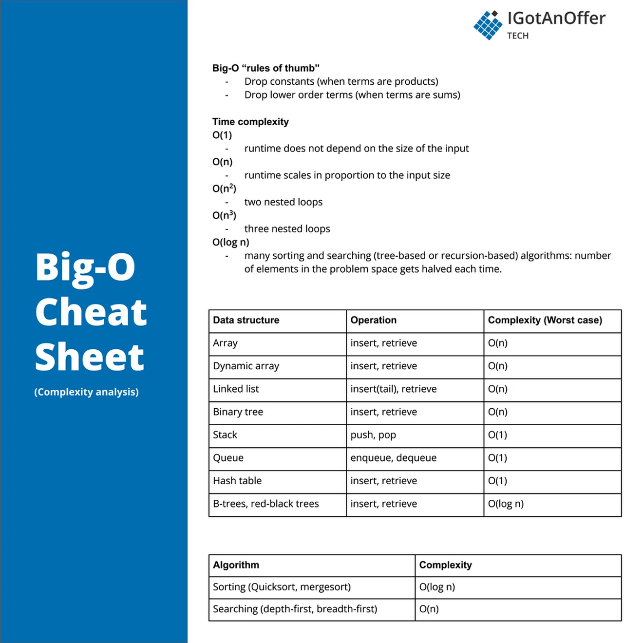
2.1 Cheat sheet for common coding structures
Here is a list of where each complexity appears the most:
- Constant time: Simple one liners, like assigning a new value to a variable, incrementing a value, or calling a function.
- Linear time: Loop or recursive calls on every element, every second element, or every nth element. This happens when visiting every element in a list, tree or graph.
- Logarithmic time: Loop or recursive calls on powers of two, half the current, other multiplication, or division. Binary search is a common division example.
- Linearithmic time: Nested loop or recursion calls of linear and logarithmic times.
- Quadratic time: Nested loop or recursion calls of linear time. A nesting level of m is a complexity of O(n^m).
- Exponential time: Recursive functions with a branching factor of b and a recursion depth of d have a complexity of O(b^d).
2.1.1 How to choose between algorithms
The cheat sheet illustrates how some tasks, like sorting, can use more than one algorithm. So which algorithm is best for a particular problem, and how do we choose between them?
Let’s compare Quicksort and mergesort as an example. The theoretical worst-case time complexity for Quicksort is O(n^2), while mergesort has a worst-case time complexity of O(n log n). At first glance, mergesort seems to be the better option.
But if we look at the space complexity of the two algorithms, Quicksort has a better space complexity at O(log n). When analyzing copy complexity, Quicksort has O(n^2) swaps, while mergesort has O(n log n). In addition, Quicksort’s average time complexity is O(n log n) and in practice we can usually ignore the theoretical worst case as it occurs only in very rare cases if the pivot is randomly chosen.
Based on these three complexities, we have to take the broader context into consideration when choosing which algorithm is best-suited. If time is our only concern, mergesort might be best.
If we are sorting on a device with limited memory (like an embedded device), then Quicksort will use less space and mergesort might not even be practical. If we are sorting data behind pointers, then the swaps won’t matter. But if we are sorting objects with heavy copy constructors, then mergesort is the better option.
The fastest algorithm is not always the best option. Consider the context of the problem you’re trying to solve and give each complexity a weighting factor appropriate to it, to arrive at a best algorithm for the context.
3. Big-O practice problems
Question 1:
If a binary search tree is not balanced, how long might it take (worst case) to find an element in it?
Solution:
O(n), where n is the number of nodes in the tree. The max time to find an element is the depth of the tree. The tree could be a straight list downwards and have depth n.
Question 2:
Work out the computational complexity of the following piece of code.
Solution:
Running time of the inner, middle, and outer loop is proportional to n, log n, and log n, respectively. Thus the overall complexity is O(n(log n)^2).
More detailed optional analysis gives the same value. Let n=2k . Then the outer loop is executed k times, the middle loop is executed k+1 times, and for each value j=2^k, 2^(k−1), ... , 2, 1, the inner loop has different execution times:
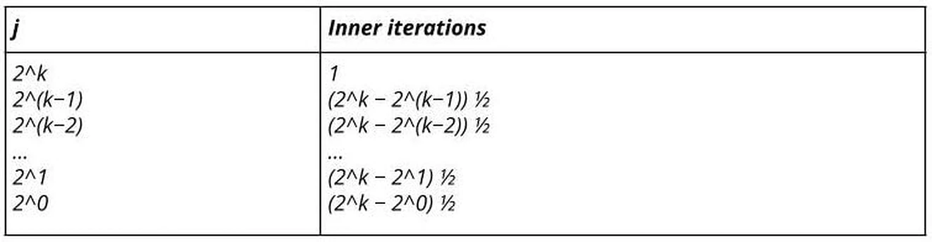
In total, the number of inner/middle steps is:
1 + k · 2^(k−1) − (1 + 2 + ... + 2^(k−1)) ½ = 1 + k · 2^(k−1) − (2^k − 1)½
= 1.5 + (k − 1) · 2^(k−1) ≡ (log2 n − 1)n/2 = O(n log n)
Thus, the total complexity is O(n(log n)^2).
Question 3:
Assume that the array a contains n values, that the method randomValue takes constant number c of computational steps to produce each output value, and that the method goodSort takes n log n computational steps to sort the array. Determine the big-O complexity for the following fragments of code, taking into account only the above computational steps:
Solution:
The inner loop has linear complexity cn, but the next called method is of higher complexity, n log n. Because the outer loop is linear in n, the overall complexity of this piece of code is O(n^(2) log n).
Question 4:
The following code sums the digits in a number. What is its big-O time?
Solution:
O(log n). The runtime will be the number of digits in the number. A number with d digits can have a value up to 10^d . If n=10^d , then d=log n.
Therefore, the runtime is O(log n).
Question 5:
The following code computes a % b. What is its runtime?
Solution:
O(1). It does a constant amount of work.
Question 6:
Consider a variation of sequential search that scans a list to return the number of occurrences of a given search key in the list. Will its efficiency differ from the efficiency of classic sequential search (O(n))?
Solution:
No. This algorithm will always make n key comparisons on every input of size n, whereas this number may vary between n and 1 for the classic version of sequential search.
Question 7:
What is the time complexity of the following code:
Solution:
The above code runs a total number of (n^2) times:
= n+(n – 1)+(n – 2)+ ... 1+0
= n*(n+1)/2
= 1/2*n^2+1/2*n
= O(n^2)
Question 8:
What is the time complexity of the following code?
Solution: O(n log n).
j keeps doubling until it is less than or equal to n, resulting in a logarithmic running time (log n). i runs for n/2 steps.
So, total time complexity :
= O(n/ 2*log (n))
= O(n log n)
Question 9:
What is the time complexity of the following code?
Solution:
O(n log n). There are log n levels, and O(n) steps are taken at each level, for a total of O(n log n)
Question 10:
What is the time complexity of the following code?
Solution:
O(nm). Let n=a_str and m=b_str. Then, the for loop is O(n). Each iteration of the for loop executes a conditional check that is, in the worst case, O(m).
Since we execute an O(m) check O(n) time, we say this function is O(nm).
4. Why big-O is important in FAANG interviews
In your day-to-day work as a software developer, you may not spend five minutes a month calculating the big-O of code written by you or others. So why do interviewers dedicate questions to big-O?
Well, because big-O should indirectly influence your choice every time you have to use a data structure when solving a problem. Engineers that don’t know data structures and the basics of big-O analysis tend to use lists to solve every problem. But we have lists, queues, stacks, maps, priority queues, map sets, graphs, and more at our disposal for solving problems.
Take building a simulation for example. An engineer that is aware of big-O will know the simulation will be dominated by insertions and deletions. The queue data structure has constant time insertion (push) and deletion (pop) complexities. So without making the connection that a simulation will have to mimic a queue, we can choose the correct data structure by just being conscious of the big-O of data structures.
Building a list of unique values is another common example. At some point, it will involve checking if the list already has an item before adding it. Using a list will have linear time complexity for checking if an item is in the list, but using a hashmap will have constant time complexity. Realizing we should use a hashmap should remind us that a hashset was designed to solve this exact problem.
Memorizing the big-Os for every data structure operation is not the best approach – nor is knowing how to implement every data structure by hand, because you will never do it.
Mastery is a better approach, since being aware of how every data structure is implemented can help you make a reasonably correct big-O estimate for any operation. And mastery enables you to eventually pick the correct data structure for problems without thinking too much about it – even during the refactoring process.
So, why do interviews include big-O questions? A smart and observant interviewer will use big-O questions to determine whether you care about the broader consequences of your code, like how well it will scale and whether it will cost the company to rework it in the future.
Your answers to big-O questions will also demonstrate how well you know data structures, proving that you’re not a developer who just hacks code together until it works without understanding why it works.
5. How to prepare for a coding interview
5.1 Refresh your knowledge
Before you start practicing interviews, you’ll want to make sure you have mastered not only complexity analysis but also the rest of the relevant algorithms and data structures. Check out our guides for detailed explanations and useful cheat sheets.
Algorithms explained:
- Depth-first search
- Breadth-first search
- Binary search
- Sorting
- Dynamic programming
- Greedy algorithm
- Backtracking
- Divide and conquer
Data structures explained:
- Arrays
- Strings
- Linked lists
- Stacks and Queues
- Graphs
- Maps
- Heap
- Coding interview examples (with solutions)
5.2 Practice on your own
Once you’re confident in all of these, you’ll want to start working through lots of coding problems.
Check out our lists of 73 data structure interview questions and 71 algorithms interview questions for practice.
One of the main challenges of coding interviews is that you have to communicate what you are doing as you are doing it. Talking through your solution out loud is therefore very helpful. This may sound strange to do on your own, but it will significantly improve the way you communicate your answers during an interview.
It's also a good idea to work on a piece of paper or google doc, given that in the real interview you'll have to code on a whiteboard or virtual equivalent.
5.3 Practice with others
Of course, if you can practice with someone else playing the role of the interviewer, that's really helpful. But sooner or later you’re probably going to want some expert interventions and feedback to really improve your coding interview skills.
That’s why we recommend practicing with ex-interviewers from top tech companies. If you know a software engineer who has experience running interviews at a big tech company, then that's fantastic. But for most of us, it's tough to find the right connections to make this happen. And it might also be difficult to practice multiple hours with that person unless you know them really well.
Here's the good news. We've already made the connections for you. We’ve created a coaching service where you can practice 1-on-1 with ex-interviewers from leading tech companies. Learn more and start scheduling sessions today.